prime number spirals
01 Oct 2014
Contents |
prime number spirals
Prime number spirals are visualizations of the distribution of prime numbers that underscore their frequent occurrences along certain polynomials. They’re conceptually simple, yet create order out of the apparent chaos of primes and are fairly beautiful. We’ll explore the Ulam and Sacks spirals, some of their underlying theory, and algorithms to render each.
Ulam spiral
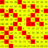
The story has it that Stanislaw Ulam, a Polish-American mathematician of thermonuclear fame1, sat in a presentation of a “long and very boring paper” at a 1963 scientific conference. After some time, he began doodling (the hallmark of great genius), first writing out the first few positive integers in a counter-clockwise spiral, and then circling all of the prime numbers. And he noticed something that he’d later formulate as “a strongly nonrandom appearance.” Even on a small scale – say, the first 121 integers, which form a 11x11 grid – it’s visible that many primes align along certain diagonal lines.
Ulam later used MANIAC II, a first-generation computer built for Los Alamos National Laboratory in 1957, to generate images of the first 65,0002 integers. The following spiral contains the first 360,000 (600x600):
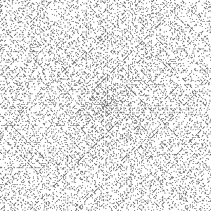
Look closely, and we see much more than just white noise.
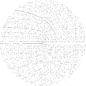
Sacks spiral
A software engineer named Robert Sacks devised a variant of the Ulam spiral in 1994. Unlike Ulam’s, Sacks’s spiral distributes integers along an Archimedean spiral, or a function of the polar form . Sacks discarded (which just controls the offset of the starting point of the curve from the pole) and used , leaving ; he then plotted the squares of all the natural numbers – – on the intersections of the spiral and the polar axis, and filled in the points between squares along the spiral, drawing them equidistant from one another.
prime-generating polynomials
The reason why we see ghostly diagonals is that some polynomials, informally called prime-generating polynomials, have aberrantly high occurrences of prime numbers. , for instance, patented by Leonhard Euler in 1772, is prime for all in the range , yielding . A variant is , proposed by Adrien-Marie Legendre in 1798, which is prime in . Here are several others, as taken at random from Wolfram Mathworld:
In the case of the rectangular Ulam spiral, these polynomials appear as diagonal lines. They were known about since 1772, if not earlier, and a prime-number spiral was hinted at twice before Ulam published his. In 1932 (31 years earlier before Ulam!), Laurence M. Klauber, a herpetologist primarily focused on the study of rattlesnakes, presented a method of using a spiral grid to identify prime-generating polynomials to the Mathematical Association of America. The second frequently-cited mention of prime spirals came from Arthur C. Clarke, a British science-fiction writer, whose The City and the Stars (1956) describes a protagonist, Jeserac, as “[setting] up the matrix of all possible integers, and [starting] his computer stringing the primes across its surface as beads might be arranged at the intersections of a mesh.” In my opinion, the second mention is fairly ambiguous, but the fact stands that, by the time Ulam published his famous spiral, a general understanding of prime-generating polynomials existed and people were considering ways of visualizing them. Thus, it’s perhaps a little disingenuous to suggest that he stumbled across it when “doodling” (something intricate) at random – there may have been some method to it.
rendering the spirals
I was introduced to prime number spirals about a year ago, by a video on the excellent Numberphile. I immediately jumped into hacking together a Python script to render the spirals on my own, because it’s both tremendously easy and very visually rewarding. I’ll revisit the implementation, this time in Javascript. I’m not going to show all of the necessary code (like HTML markup/CSS styles) in the interest of brevity, but the zipped files are linked to at the end of the post.
canvas setup
Let’s outline our interface. We’ll define functions ulamSpiral(numLayers) and sacksSpiral(numLayers), where
the argument numLayers is the number of revolutions in the spiral, or effectively the number of rings that it contains. Both
functions need to set the height and width of the canvas according to numLayers, and require a function
drawPixel(x, y) to plot pixels. Note that we’ll want drawPixel() to treat the centroid of the canvas as its
origin, so that drawPixel(0, 0) plots a point at its center and not the top-left corner. Because both the canvas
dimensions and the offset used by drawPixel() are dependent on numLayers, we’ll bundle them them into a function
called setupCanvas().
function setupCanvas(numLayers){
	"use strict";

	var sideLen = numLayers * 2 + 1;
	var canvas = document.getElementsByTagName("canvas")[0];
	canvas.setAttribute("width", sideLen);
	canvas.setAttribute("height", sideLen);

	var context = canvas.getContext("2d");
	return function drawPixel(x, y){
		context.fillRect(x + numLayers, y + numLayers, 1, 1);
	};
}
Note that we set sideLen equal to numLayers * 2 + 1, rather than only numLayers * 2, because we need to account for the
row/column containing the origin of the spiral, which is not technically a ring. Now, we can use setupCanvas() to
both set the canvas dimensions, and return a drawPixel() that takes advantage of closure to access all of the
variables (numLayers, context) that it needs. Also, to draw a single pixel, we’re calling fillRect() with a
width and height of 1 – the canvas unfortunately doesn’t have (or perhaps just doesn’t expose) a single pixel-plotting
function. Finally, to test the primality of our values, we’ll use Kenan Yildirim’s
primality library, which provides primality(val).
Ulam algorithm
The dull stuff aside, we can begin implementing ulamSpiral(). The general algorithm will run as follows:
- Use variables
x,y, andcurrValueto track the position and value of the current point – the “head” of the spiral. - Trace out the square spirals by incrementing/decrementing
xandy, while incrementingcurrValue. - After the head of the spiral moves, if
currValueis prime, plot a pixel at (x,y).
function ulamSpiral(numLayers){
	"use strict";

	var drawPixel = setupCanvas(numLayers);

	var currValue = 1;
	var x = 0;
	var y = 0;

	function drawLine(dx, dy, len){
		for(var pixel = 0; pixel < len; pixel++){
			if(primality(currValue++)){
				drawPixel(x, y);
			}
			x += dx;
			y += dy;
		}
	}

	for(var layer = 0, len = 0; layer <= numLayers; layer++, len += 2){
		drawLine(0, -1, len - 1);
		drawLine(-1, 0, len);
		drawLine(0, 1, len);
		drawLine(1, 0, len + 1);
	}
}
We simply iterate numLayers + 1 times, drawing rectangular layers – the spiral – as we go. I couldn’t think of a
better solution than using a function drawLine(), which accepts a direction (dx and dy, one of which should be
0), and a length to draw four different straight lines (perhaps it can somehow be done in one elegant loop?).
Sacks algorithm
The Sacks spiral is a little more mathematically interesting because it relies (somewhat) on polar equations. Our algorithm:
- Iterate
numLayerstimes. - For each iteration, draw the values between the current square, , and the next, . Since , there are points per iteration of .
- Render each prime point by calculating its angle off the polar axis (the aligned squares), then its radius, or distance from the pole, and then using trigonometry to solve for its cartesian coordinates.
function sacksSpiral(numLayers){
	"use strict";

	var drawPixel = setupCanvas(numLayers);

	var currValue = 1;
	for(var layer = 1; layer <= numLayers; layer++){
		var numPoints = 2 * layer + 1;
		var angle = 2 * Math.PI / numPoints;
		for(var point = 1; point <= numPoints; point++){
			if(primality(currValue++)){
				var theta = point * angle;
				var radius = layer + point / numPoints;
				var x = Math.cos(theta) * radius;
				var y = Math.sin(theta) * radius;
				drawPixel(Math.floor(x), Math.floor(y));
			}
		}
	}
}
To calculate the polar angle of any point, we first solve for the angle between subsequent points
(var angle = 2 * Math.PI / numPoints;), and then multiply it by the fraction of the current rotation of the spiral
that the point lies at (var theta = point * angle;). We’ll also Math.floor() the coordinates sent to drawPixel(),
because, after the various trigonometic operations they’re likely decimals rather than integers and cause blurred
canvas reading.
That’s all! For more reading on prime-number spirals, I recommend this in-depth article by Robert Sacks himself, and another write-up of algorithms used to render them.
Download all of the source code here, or view it on Github.
-
Ulam is also well-known for contributing to the Manhattan Project, proponing the Monte Carlo method of computation, and exploring spaceships propelled by nuclear explosions, amongst a large number of other things. ↩
-
Assuming that Ulam began rendering his spiral with the integer 1 (instead of something like 41, which is also common), I suspect that the generated images had exactly 65,025 integers. 65,000 integers implies as many pixels, the square root – the Ulam spiral is inherently square – of which is 254.95, which obviously isn’t a valid image height/width. Thus, we round to 255, and square for 65,025. ↩